🎉 Success! You're now signed up for the Shakudo newsletter.
Oops! Something went wrong while submitting the form.
Congratulations, your business is up and running! You have an attractive array of services with happy customers ready to pay for them - and very few of them are scamming you! But being the go-getter that you are, you're striving for more - to reach for the eternal dream, the Elysium fields where even fewer customers are committing fraud. Let's figure out how you can find instances of fraud.
When you have a large amount of complex data to categorize, such as labeling a database of customer transactions as "fraudulent" or "not fraudulent", you’ll likely want to employ a machine learning solution. Human intervention is slow and costly, while bespoke "expert system" solutions are expensive to build, questionably accurate, and need to be manually updated any time the behavior behind your data changes (eg. fraudsters adopting new tactics).
Meanwhile, if built well, machine learning approaches will improve in accuracy and adapt to systemic changes if you throw more and newer data at them. They also scale well with both absolute data volume and with data throughput - you don't want this system to become a transaction bottleneck as you expand to serve more customers.
Great - this is the point where you pick out some models and begin training.
Unfortunately, this is also the point where you run into a classic bootstrapping problem. All the models you’ll find need to train using a labeled dataset - and if you had an easy way of labeling your data, you wouldn't be looking for a model in the first place. Unless you're working with a longstanding company that already has a large backlog of fraud cases, it'll start to look like you won't be able to train your model to find fraud at all.
Fortunately, rather than solving this problem directly, you can cheat. You can trust the panglossian assumption that fraud is rare*, and rather than teaching the model to find fraud, you’ll teach it to find strange and anomalous occurrences - which we can then cynically assume are most likely fraud.
This process does rely on the assumption that data collected from honest and fraudulent transactions will follow different distributions. If there actually is no detectable difference between the two, then nothing will be able to find the fraud, and you’ll need to start collecting better data. Luckily, anomaly detection is a commonly used fraud detection method with a great track record.
I always say the absence of evidence is not the evidence of absence. Simply because you don't have evidence that something does exist does not mean you have evidence of something that doesn't exist. [...] What I'm saying is that there are known knowns and that there are known unknowns. But there are also unknown unknowns; things we don't know that we don't know. -- Gin Rummy, The Boondocks
A comprehensive review of all anomaly detection methods is well beyond the scope of this blog post, so we will be focusing on one effective (and broadly applicable) method: autoencoder reconstruction error. We will also make available the accompanying Python notebook on the Shakudo sandbox under ~/gitrepo/anomaly_fraud_detection/unsupervised_anomaly_detection.ipynb. Sign up now for a free account and test it out yourself!
An autoencoder is a neural net with two parts: one to compress (encode) data into a more compact representation, and the second to decompress (decode) that back into the original form. This works for many different types of data, as the information content of a real-world dataset is often smaller than what its feature space is capable of containing.
To train an autoencoder you’ll create a neural net such that the input and output layers both have a number of nodes equal to the size of our feature set, with a smaller hidden layer somewhere in between. The representation of the data within the smallest layer is called the "code" or “latent representation”. The group of all layers from input to code is the encoder, and the group of layers from code to output is the decoder. From there, you define the loss function as the mean squared error of the output compared to the input, and you’re ready to train.
In this example we’ll use Tensorflow, but any modern deep learning library will be similarly capable. You can either set up the necessary hardware and software yourself, or try a managed dev environment. If you have the time you can always build everything from scratch, but often it's more convenient to write 20 lines of code in a managed workspace instead.
For many autoencoder applications, you’ll want to use a code layer large enough that the reconstruction error is negligible. Here we’re using one significantly smaller than that. By intentionally limiting the code size we force errors to happen, and given data with vastly imbalanced category sizes (and no class-weighting), the most common category overwhelms the others and effectively causes the network to not learn them. This means that, after training, high reconstruction error for a given datapoint will suggest that it is abnormal in some way.
Example Data
For our example we will use data from the Credit Card Fraud Detection Kaggle competition. It’s a labeled dataset, so the first thing we’ll do after importing it is remove those labels and set them aside for later verification.
The data has already been anonymized via PCA transformation. This means there isn't much to see when you look at the data yourself, so we'll skip the usual preliminary data examination. PCA can also result in dimensionality reduction in a somewhat similar manner to autoencoders, so this may reduce the effectiveness of our approach. Unfortunately most of the large databases of non-anonymized credit card transactions available online are not quite legal enough for this sort of blog, so we'll have to work with the example data we have.
We’ll normalize the data and convert it to a tensor, and then it's time to train the model:
In most circumstances it's necessary to split your data into training and validation subsets, as network accuracy can't be trusted when evaluated on the same data used for training. It's not strictly necessary in this case, however, because there is no label for the network to memorize. Splitting the data could even be risky: the low number of fraud examples means the two datasets could end up with very different concentrations, and without labels there would be no way to enforce balance. Adding this data split could be a fun test, though, and we encourage you to try it out on Shakudo.
Analyzing Your Results
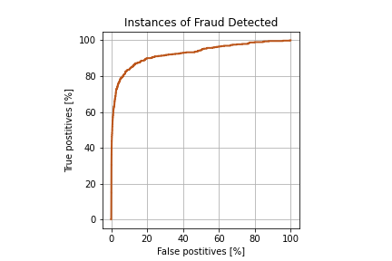
Time to bring out the labels and see how they match up to our error-based suspicion metric. First we'll plot the receiver operating characteristic curve, in which we vary the error threshold above which fraud is assumed, and plot the resulting number of true and false positives:
Looks pretty good for an attempt to find hidden events we knew nothing about, simply by assuming "they're probably different". We’re finding 60% of all fraud with a false positive rate of around 1%! Which sounds fantastic, until you remember the extreme data imbalance.
Total honest transactions: 284,315
Total fraudulent transactions: 492
That means that our seemingly solid conclusions actually correspond to 296 cases of fraud with 3,392 false positives - reducing the precision to 8% at that threshold. Still an improvement from the base random chance rate of 0.17%, but not as impressive as it seems at first glance.
These results are far from worthless, though. When we examine the accuracy for the most suspicious transactions, corresponding to the lower left region of the ROC curve, we see a much higher success rate:
Here there’s roughly 33% precision for several hundred of the most suspicious transactions. This is high enough that you could employ this method to trigger manual investigation and confirmation, not only preventing lost money with each real case of fraud found, but also forming the beginning of a labeled dataset. And realistically, even with a very accurate model you would still want a human in the loop somewhere for a serious matter like accusations of fraud. The alternative can be concerning.
Looking forward, once you've investigated enough cases, it'll be time to revisit this model and improve its accuracy by splicing it into a semi-supervised system - but that's a topic for a later article.
* If a very large fraction of your customers are thieves this probably won’t work. In that case, look forward to our upcoming article about clustering!
Ian Watt
Ian Watt earned his Masters of Engineering from McGill University for work in deep reinforcement learning for medical image registration and his Bachelors in Mechatronics Engineering from Western University. Prior to joining Shakudo, Ian worked on projects in bioinformatics, robotics, and 3d printing.
| Case Study
Anomaly Detection: Using Machine Learning to Find Fraud
Key results
About
industry
Data Stack
No items found.
Congratulations, your business is up and running! You have an attractive array of services with happy customers ready to pay for them - and very few of them are scamming you! But being the go-getter that you are, you're striving for more - to reach for the eternal dream, the Elysium fields where even fewer customers are committing fraud. Let's figure out how you can find instances of fraud.
When you have a large amount of complex data to categorize, such as labeling a database of customer transactions as "fraudulent" or "not fraudulent", you’ll likely want to employ a machine learning solution. Human intervention is slow and costly, while bespoke "expert system" solutions are expensive to build, questionably accurate, and need to be manually updated any time the behavior behind your data changes (eg. fraudsters adopting new tactics).
Meanwhile, if built well, machine learning approaches will improve in accuracy and adapt to systemic changes if you throw more and newer data at them. They also scale well with both absolute data volume and with data throughput - you don't want this system to become a transaction bottleneck as you expand to serve more customers.
Great - this is the point where you pick out some models and begin training.
Unfortunately, this is also the point where you run into a classic bootstrapping problem. All the models you’ll find need to train using a labeled dataset - and if you had an easy way of labeling your data, you wouldn't be looking for a model in the first place. Unless you're working with a longstanding company that already has a large backlog of fraud cases, it'll start to look like you won't be able to train your model to find fraud at all.
Fortunately, rather than solving this problem directly, you can cheat. You can trust the panglossian assumption that fraud is rare*, and rather than teaching the model to find fraud, you’ll teach it to find strange and anomalous occurrences - which we can then cynically assume are most likely fraud.
This process does rely on the assumption that data collected from honest and fraudulent transactions will follow different distributions. If there actually is no detectable difference between the two, then nothing will be able to find the fraud, and you’ll need to start collecting better data. Luckily, anomaly detection is a commonly used fraud detection method with a great track record.
I always say the absence of evidence is not the evidence of absence. Simply because you don't have evidence that something does exist does not mean you have evidence of something that doesn't exist. [...] What I'm saying is that there are known knowns and that there are known unknowns. But there are also unknown unknowns; things we don't know that we don't know. -- Gin Rummy, The Boondocks
A comprehensive review of all anomaly detection methods is well beyond the scope of this blog post, so we will be focusing on one effective (and broadly applicable) method: autoencoder reconstruction error. We will also make available the accompanying Python notebook on the Shakudo sandbox under ~/gitrepo/anomaly_fraud_detection/unsupervised_anomaly_detection.ipynb. Sign up now for a free account and test it out yourself!
An autoencoder is a neural net with two parts: one to compress (encode) data into a more compact representation, and the second to decompress (decode) that back into the original form. This works for many different types of data, as the information content of a real-world dataset is often smaller than what its feature space is capable of containing.
To train an autoencoder you’ll create a neural net such that the input and output layers both have a number of nodes equal to the size of our feature set, with a smaller hidden layer somewhere in between. The representation of the data within the smallest layer is called the "code" or “latent representation”. The group of all layers from input to code is the encoder, and the group of layers from code to output is the decoder. From there, you define the loss function as the mean squared error of the output compared to the input, and you’re ready to train.
In this example we’ll use Tensorflow, but any modern deep learning library will be similarly capable. You can either set up the necessary hardware and software yourself, or try a managed dev environment. If you have the time you can always build everything from scratch, but often it's more convenient to write 20 lines of code in a managed workspace instead.
For many autoencoder applications, you’ll want to use a code layer large enough that the reconstruction error is negligible. Here we’re using one significantly smaller than that. By intentionally limiting the code size we force errors to happen, and given data with vastly imbalanced category sizes (and no class-weighting), the most common category overwhelms the others and effectively causes the network to not learn them. This means that, after training, high reconstruction error for a given datapoint will suggest that it is abnormal in some way.
Example Data
For our example we will use data from the Credit Card Fraud Detection Kaggle competition. It’s a labeled dataset, so the first thing we’ll do after importing it is remove those labels and set them aside for later verification.
The data has already been anonymized via PCA transformation. This means there isn't much to see when you look at the data yourself, so we'll skip the usual preliminary data examination. PCA can also result in dimensionality reduction in a somewhat similar manner to autoencoders, so this may reduce the effectiveness of our approach. Unfortunately most of the large databases of non-anonymized credit card transactions available online are not quite legal enough for this sort of blog, so we'll have to work with the example data we have.
We’ll normalize the data and convert it to a tensor, and then it's time to train the model:
In most circumstances it's necessary to split your data into training and validation subsets, as network accuracy can't be trusted when evaluated on the same data used for training. It's not strictly necessary in this case, however, because there is no label for the network to memorize. Splitting the data could even be risky: the low number of fraud examples means the two datasets could end up with very different concentrations, and without labels there would be no way to enforce balance. Adding this data split could be a fun test, though, and we encourage you to try it out on Shakudo.
Analyzing Your Results
Time to bring out the labels and see how they match up to our error-based suspicion metric. First we'll plot the receiver operating characteristic curve, in which we vary the error threshold above which fraud is assumed, and plot the resulting number of true and false positives:
Looks pretty good for an attempt to find hidden events we knew nothing about, simply by assuming "they're probably different". We’re finding 60% of all fraud with a false positive rate of around 1%! Which sounds fantastic, until you remember the extreme data imbalance.
Total honest transactions: 284,315
Total fraudulent transactions: 492
That means that our seemingly solid conclusions actually correspond to 296 cases of fraud with 3,392 false positives - reducing the precision to 8% at that threshold. Still an improvement from the base random chance rate of 0.17%, but not as impressive as it seems at first glance.
These results are far from worthless, though. When we examine the accuracy for the most suspicious transactions, corresponding to the lower left region of the ROC curve, we see a much higher success rate:
Here there’s roughly 33% precision for several hundred of the most suspicious transactions. This is high enough that you could employ this method to trigger manual investigation and confirmation, not only preventing lost money with each real case of fraud found, but also forming the beginning of a labeled dataset. And realistically, even with a very accurate model you would still want a human in the loop somewhere for a serious matter like accusations of fraud. The alternative can be concerning.
Looking forward, once you've investigated enough cases, it'll be time to revisit this model and improve its accuracy by splicing it into a semi-supervised system - but that's a topic for a later article.
* If a very large fraction of your customers are thieves this probably won’t work. In that case, look forward to our upcoming article about clustering!
Use data and AI products inside your infrastructure
Chat with one of our experts to answer your questions about your data stack, data tools you need, and deploying Shakudo on your cloud.


.svg)

.jpg)
.svg)
.jpg)


